|
Alpine3D 20240419.cd14b8b
|


|
|
Alpine3D 20240419.cd14b8b
|
|
When running a simulation, it is important to keep in mind that the model is organized as several modules that interract together. It is possible to configure some parameters for the various modules and to enable/disable modules. Some modules can be used outside of Alpine3D (like MeteoIO that is used in various applications or libSnowpack that is used by the standalone Snowpack model) .

Please follow the instructions given on the forge in order to download Alpine3D (from git, from source or from a binary package) and its dependencies (Snowpack and MeteoIO, knowing that binary packages might already contain all the required dependencies). If you've downloaded a binary package, there is nothing special to do, just install it on your system.
When installing Alpine3D from sources, please keep in mind that Alpine3D's compilation process is exactly the same as Snowpack's or MeteoIO's (all are based on cmake). After a successful compilation, it is necessary to install Alpine3D (the same must have been done for Snowpack and MeteoIO). There are two options:
After Alpine3D has been installed, you can check that it works by opening a terminal and typing "alpine3d". Alpine3D should be found and display its help message.
After you installed a binary package or compiled and installed Alpine3D (on most compute clusters, you will need to install in your own home directory, see installing Alpine3D above), you can run your first simulation. We highly recommend that you use the following structure: first, create a directory for your simulation, for example "Stillberg". Then, create the following sub-directories:
Edit the "run.sh" script to set it up with the proper start and end dates, the modules that you want to enable and the proper configuration for a sequential or parallel run.
This is the simplest way of running an Alpine3D simulation: it runs on one core on one computer. The drawback is that if the simulation is quite large, it might require a very long time to run or even not have enough memory (RAM) to run once there is snow in the simulated domain. In order to run a sequential simulation, set "PARALLEL=N" in the run.sh script. Then run the following command in a terminal (this can be a remote terminal such as ssh) on the computer where the simulation should run:
nohup means that if you close the terminal the simulation will keep going; & means that the terminal prompt can acept other commands after you've submitted this one. In order to monitor what is going on with your simulation, simply run something such as (-f means that it keeps updating with the new content in this file. Replace it with something such as -500 to show the last 500 lines of this file):
If you need to terminate the simulation, first find out its Process ID (PID) by doing
Then kill the process
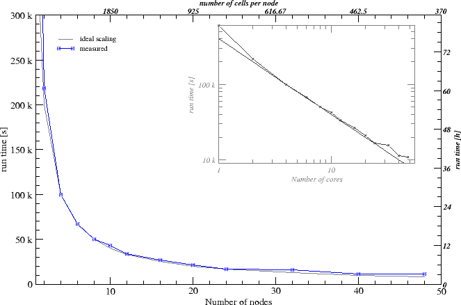
When a simulated domain gets bigger, the computational requirements (memory and runtime) get bigger. In order to reduce these requirements, it is possible to run the simulation in parallel accross multiple cores or nodes.
This is the easiest way to run a parallel simulation because it does not require any specific software, only a compiler that supports OpenMP (see also its wikipedia page). Such compilers are for example gcc, clang, etc. The limitations on the memory still remain (ie a simulation requiring lots of memory will still only have access to the local computer's memory) but the run time will be roughtly divided by the number of available cores that are given to the simulation. In order to run such a simulation, please compile Alpine3D with the OpenMP option set to ON in cmake. Then in the simulation's run.sh file, set "PARALLEL=OPENMP" as well as the number of cores you want to us as "NCORES=". Then run the simulation as laid out in the previous section.
This is the most powerful way of running a simulation: the load is distributed among distinct computing nodes, therefore reducing the amount of memory that must be available on each node. For very large simulations, this might be the only way to proceed. This is achieved by relying on MPI to exchange data between the nodes and distribute the workload. In order to run such a simulation, please compile Alpine3D with the MPI option set to ON in cmake. Then in the simulation's run.sh file, set "PARALLEL=MPI" as well as the number of processors/cores you want to us as "NPROC=" and a machine file. This machine file contains the list of machines to use for the simulation as well as how many processors/cores to use. For example, such as file could be:
Then run the simulation as laid out in the previous section.
If your computing infrastructure relies on Sun/Oracle Grid Engine (SGE) (for example on a computing cluster), you need to do things differently. First, the job management directives/options must be provided, either on the command line or in the run.sh script. These lines rely on special comments, starting with "#" followed by "$":
The last line specifies the computing profile that should be used. Since the job manager will allocate the ressources, there is no need to provide either NCORES or NPROC. The machine file (for MPI) is also not used. Then, submit the computing job to the system: "qsub ./run.sh". This should return almost immediately with a message providing the allocated job number. This job number is useful to delete the job "qdel {job_number}" or querry its status "qstat {job_number}" (or "qstat" to see for all jobs).
If the job submission fails with an error message such as unknown command, please check that there is no extra "#$" in the script. This happens frequently when commenting out some part of the script and is mis-interpreted by SGE. In such a case, simply add an extra "#" in front of the comment.
Depending on the meteorological data availability, the meteorological data quality as well as convenience (if the raw data is difficult to access, for example), there are different data strategies that can be used. This is illustrated in the figure below.
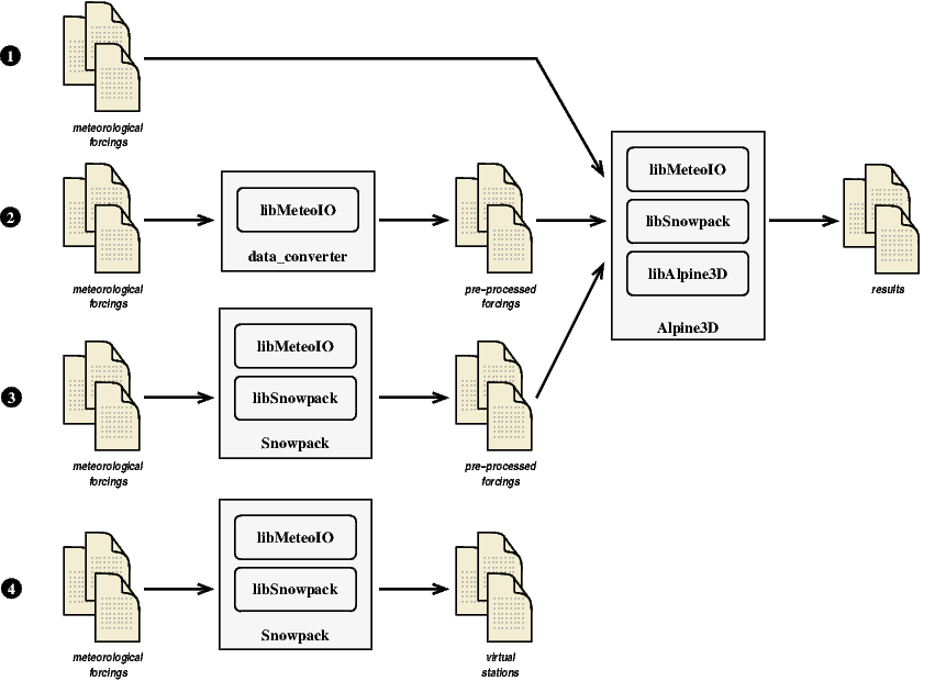
The simplest case is 1: the meteorological forcings are directly read and processed by Alpine3D. Since it embbeds MeteoIO, it can perform the whole preprocessing on the fly. In order to have a look at the pre-processed data (or to spare a lengthy data extraction), it is possible to preprocess the data first, then dump them to files and run Alpine3D from these intermediate file (case 2). Since Alpine3D anyway embbeds MeteoIO, it would be possible to add some pre-processing to be done on the fly within Alpine3D (such as resampling to the sampling rates that Alpine3D needs). This is actually highly recommended in order to guarantee that Alpine3D gets the data it needs (ie proper sampling rates as well as basic checks on the ranges, etc).
In some cases, it might be interesting to first run the data through Snowpack in order to produce some meteorological parameter from other parameters, such as the ISWR from RSWR (since Snowpack computes the snow albedo, the generate data would be much better than assuming a fixed albedo) or to generate precipitation from the measured snow height. This is shown in case 3.
Case 4 shows a strategy that could be used to prepare an Alpine3D simulation: it consists of simple Snowpack simulations performed at spatially interpolated locations, using MeteoIO's virtual stations concept. This is useful to (relatively) quickly validate the spatially interpolated fields with some measured data (specially if there are some meteorological data that could be compared to the spatially interpolated meteorological fields).
Alpine3D needs spatially interpolated forcings for each grid points. Unfortunately, it limits the choice of forcing parameters: for some parameters (such as HS or RSWR), there are no reliable interpolation methods. One way to make use of the existing measurements that could not be easily interpolated is to run a Snowpack simulation at the stations that provided these measurements, then use alternate, computed parameters (such as PSUM or ISWR) as inputs to Alpine3D.
This process is made easier by writing Snowpack's outputs in the smet format and making sure all the necessary parameters are written out. This means that Snowpack should be configured along the following lines (only using one slope):
Then the output smet files produced by Snowpack can be directly used as Alpine3D inputs, performing some on-the-fly renaming and conversions (here, from split precipitation to precipitation/phase):
Of course, other stations can also be part of the meteo input and their inputs should remain unaffected (assuming they don't use parameter names such as MS_Snow, MS_Rain or HS_meas and assuming that their parameters are not rejected by the KEEP command). As a side note, the last three parameter renamings (with MOVE) must be set when using Snowpack's outputs as inputs for a new Snowpack simulation.